Your First Plot with Biggles

The easiest way to start plotting with biggles is to use the convenience functions:

from biggles import plot

plot(x, y)

See the documentation here.

Jupyter Notebooks

If you are working in a jupyter notebook, simply typing the name of the plot object (returned by the function above or you can declare one below) and enter will produce an inline plot. You can control the resolution of the inline plot by setting the dpi attribute.

p.dpi=100
p

The Object-Oriented Interface

For more complicated plots, biggles has a simple, object-oriented interface. You declare containers and then add components to them. Let's make out first plot with biggles!

First, you instantiate a container. In this example, we will use a FramedPlot.

import biggles

p = biggles.FramedPlot()

We can set axis ranges, aspect ratios (and other properties) of the FramedPlot using its attributes:

p.xrange = 0, 100
p.yrange = 0, 100
p.aspect_ratio = 1

Now, let's make some data to plot:

import numpy
x = numpy.arange(0, 100, 5)
yA = numpy.random.normal(40, 10, (len(x),))
yB = x + numpy.random.normal(0, 5, (len(x),))

We can add this data to the plot by instantiating Points objects:

a = biggles.Points(x, yA, type="circle")
a.label = "a points"

b = biggles.Points(x, yB)
b.label = "b points"
b.style(type="filled circle")

Notice here we have set labels for the points and have used the style method to set the style of the points. See the documentation to see all of the style options.

Let's instantiate a Slope component to use for data annotation:

l = biggles.Slope(1, type="dotted")
l.label = "slope"

Further, we would like a PlotKey for our labels:

k = biggles.PlotKey(.1, .9)
k += a, b, l

Finally, let's add these components to the plot, display it in an X window, and then write a copy to disk:

p += l, a, b, k
p.show()
p.write("example.pdf")

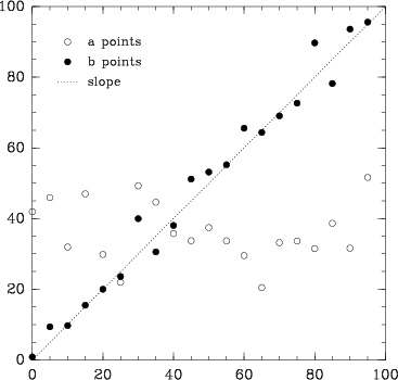
These steps will produce a plot that looks like this:

Next Steps

This example showcases only a small fraction of what biggles can do. See the Reference Guide and the examples for more information.